QuantStudio3 Uniformity Test
Rationale
Testing the new QuantStudio3 machine for any potential variation among wells using a plate with 96 technical replicates, i.e., the same reaction in each well, that includes amplification of both C and D actin loci (VIC and FAM dyes, respectively).
Methods
- Prepare DNA template: (200 µL total)
- 100 µL clade C actin @ 64,000 copies/µL
- 100 µL clade D actin @ 64,000 copies/µL
- Prepare qPCR MasterMix:
- Each reaction: 5 µL GTMM; 0.5 µL each of CFor, CRev, CProbe(VIC), DFor, DRev, DProbe(FAM); (no water)
- MasterMix (n=98): 490 µL GTMM; 49 µL each oligo
- Add 8 µL MasterMix to each well
- Add 2 µL mixed C+D DNA template to each well
Results
Raw data files:
library(reshape2)
df <- read.delim("2018-01-23_Uniformity-Test.txt", skip=7923, sep="\t")
df <- dcast(df, formula=Well.Position~Target.Name, value.var="CT")
Visualize plates:
library(platetools)
raw_map(data=df$C, well=df$Well, plate=96)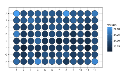
raw_map(data=df$D, well=df$Well, plate=96)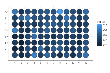
Run some stats:
library(effects)
library(lsmeans)
## Loading required package: estimability## Loading required package: methodsdf$row <- factor(substr(df$Well, 1,1))
df$col <- factor(as.numeric(substr(df$Well, 2,3)))
df$corner <- factor(ifelse(df$Well %in% c("A1", "A12", "H1", "H12"), "corner", "not_corner"))
df$border <- factor(ifelse(df$row %in% c("A", "H") | df$col %in% c(1, 12), "border", "not_border"))
str(df)## 'data.frame': 96 obs. of 7 variables:
## $ Well.Position: Factor w/ 96 levels "A1","A10","A11",..: 1 2 3 4 5 6 7 8 9 10 ...
## $ C : num 24.6 24.1 24.1 24.3 24 ...
## $ D : num 24.4 24.2 24 24.3 24 ...
## $ row : Factor w/ 8 levels "A","B","C","D",..: 1 1 1 1 1 1 1 1 1 1 ...
## $ col : Factor w/ 12 levels "1","2","3","4",..: 1 10 11 12 2 3 4 5 6 7 ...
## $ corner : Factor w/ 2 levels "corner","not_corner": 1 2 2 1 2 2 2 2 2 2 ...
## $ border : Factor w/ 2 levels "border","not_border": 1 1 1 1 1 1 1 1 1 1 ...# Are corners different?
mod <- lm(C ~ corner, data=df)
pairs(lsmeans(mod, specs="corner"))## contrast estimate SE df t.ratio p.value
## corner - not_corner 0.4512174 0.08782635 94 5.138 <.0001plot(effect("corner", mod), main="Corner effect - C assay")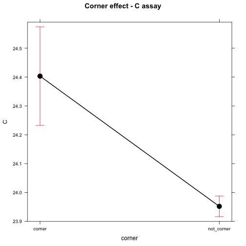
mod <- lm(D ~ corner, data=df)
pairs(lsmeans(mod, specs="corner"))
## contrast estimate SE df t.ratio p.value
## corner - not_corner 0.1955435 0.07748637 94 2.524 0.0133plot(effect("corner", mod), main="Corner effect - D assay")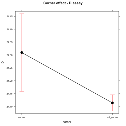
# Are columns different? (excluding corners)
mod <- lm(C ~ col, data=subset(df, corner=="not_corner"))
anova(mod)
## Analysis of Variance Table
##
## Response: C
## Df Sum Sq Mean Sq F value Pr(>F)
## col 11 0.36627 0.033297 1.1377 0.3441
## Residuals 80 2.34145 0.029268plot(effect("col", mod), main="Column effect - C assay (excluding corners)")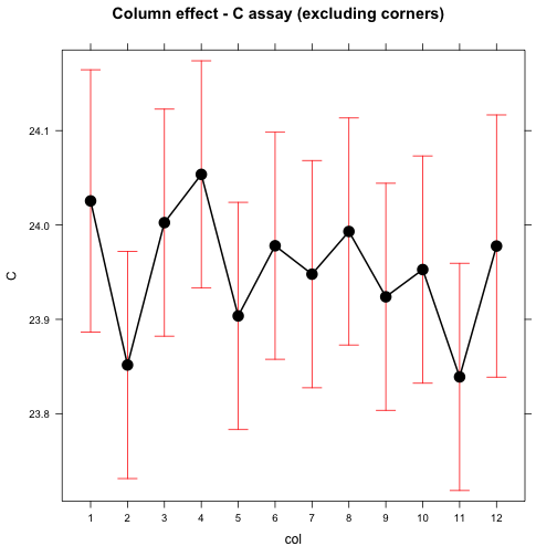
mod <- lm(D ~ col, data=subset(df, corner=="not_corner"))
anova(mod)
## Analysis of Variance Table
##
## Response: D
## Df Sum Sq Mean Sq F value Pr(>F)
## col 11 0.5442 0.049473 2.5245 0.008732 **
## Residuals 80 1.5677 0.019597
## ---
## Signif. codes: 0 '***' 0.001 '**' 0.01 '*' 0.05 '.' 0.1 ' ' 1plot(effect("col", mod), main="Column effect - D assay (excluding corners)")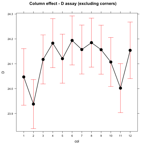
# Are rows different? (excluding corners)
mod <- lm(C ~ row, data=subset(df, corner=="not_corner"))
anova(mod)
## Analysis of Variance Table
##
## Response: C
## Df Sum Sq Mean Sq F value Pr(>F)
## row 7 1.0537 0.15053 7.645 4.027e-07 ***
## Residuals 84 1.6540 0.01969
## ---
## Signif. codes: 0 '***' 0.001 '**' 0.01 '*' 0.05 '.' 0.1 ' ' 1cld(lsmeans(mod, specs="row"))## row lsmean SE df lower.CL upper.CL .group
## F 23.79792 0.04050762 84 23.71736 23.87847 1
## E 23.83150 0.04050762 84 23.75095 23.91205 1
## D 23.92058 0.04050762 84 23.84003 24.00114 12
## G 23.92608 0.04050762 84 23.84553 24.00664 12
## C 23.93683 0.04050762 84 23.85628 24.01739 12
## H 24.05800 0.04437388 84 23.96976 24.14624 23
## B 24.06542 0.04050762 84 23.98486 24.14597 23
## A 24.12670 0.04437388 84 24.03846 24.21494 3
##
## Confidence level used: 0.95
## P value adjustment: tukey method for comparing a family of 8 estimates
## significance level used: alpha = 0.05plot(effect("row", mod), main="Row effect - C assay (excluding corners)")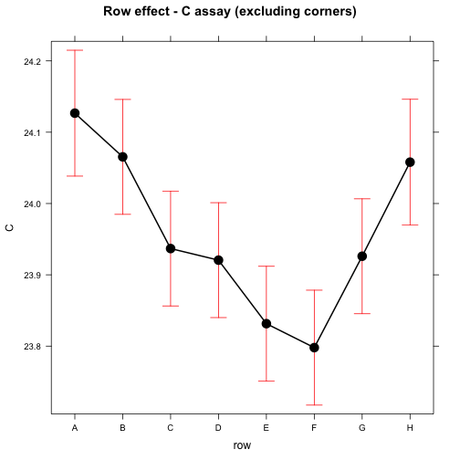
mod <- lm(D ~ row, data=subset(df, corner=="not_corner"))
anova(mod)
## Analysis of Variance Table
##
## Response: D
## Df Sum Sq Mean Sq F value Pr(>F)
## row 7 0.32654 0.046648 2.1947 0.04268 *
## Residuals 84 1.78542 0.021255
## ---
## Signif. codes: 0 '***' 0.001 '**' 0.01 '*' 0.05 '.' 0.1 ' ' 1cld(lsmeans(mod, specs="row"))## row lsmean SE df lower.CL upper.CL .group
## F 24.02392 0.04208617 84 23.94022 24.10761 1
## E 24.05117 0.04208617 84 23.96747 24.13486 1
## G 24.09233 0.04208617 84 24.00864 24.17603 1
## C 24.09558 0.04208617 84 24.01189 24.17928 1
## H 24.11900 0.04610309 84 24.02732 24.21068 1
## D 24.14767 0.04208617 84 24.06397 24.23136 1
## A 24.19000 0.04610309 84 24.09832 24.28168 1
## B 24.20550 0.04208617 84 24.12181 24.28919 1
##
## Confidence level used: 0.95
## P value adjustment: tukey method for comparing a family of 8 estimates
## significance level used: alpha = 0.05plot(effect("row", mod), main="Row effect - D assay (excluding corners)")
Conclusions:
Detection in the corners is 0.45 cycles later for C (VIC) and 0.2 cycles later for D (FAM).
There is a significant column effect for D (FAM) detection.
There is a significant row effect for C (VIC) detection.