Rationale

Test amplification success and efficiency of new primers targeting Platygyra Pax-C intron.
Test for presence of inhibitors in KI Platygyra DNA samples.
Test whether PowerUp SYBR MasterMix is more robust to inhibitors.

Methods

Samples used:
- KI15aFSYM097 (2015a-097): [DNA] = 22.1 ng/µL
- KI16aFSYM108 (2016a-108): [DNA] = 9.28 ng/µL
- Prepare log10 dilution series of each sample: 1:5, 1:50, 1:500, 1:5000, 1:50000
Primers used:
- Platy_Pax-C_F1 (5’-GGATACCCGCGTCGACTCT-3’)
- Platy_Pax-C_R1 (5’-CCCTAAGTTTGCTTTTTATTGTTCCT-3’)
Prepare qPCR MasterMixes:
- Each reaction: 6.25 µL SYBR, 0.1125 µL each primer @ 100 µM, 4.025 µL water, 2 µL template DNA
- MasterMix (n=22): 137.5 µL SYBR, 2.475 µL each primer @ 100 µM, 88.55 µL water –> 10.5 µL each well
  - make two MMs, one containing SYBR Green, one containing PowerUp SYBR

Results

Raw data files:

library(reshape2)
library(stringr)

## Warning: package 'stringr' was built under R version 3.3.2

df <- read.delim("RC_20171010_PlatyPaxC_primertest_data.txt", skip=8)[, 1:7]
df <- df[df$Target.Name=="PaxC1", ]
df$CT <- as.numeric(as.character(df$Cт))

## Warning: NAs introduced by coercion

df$col <- substr(df$Well, 2, 3)
df$row <- substr(df$Well, 1, 1)
df$MM <- factor(ifelse(df$col %in% 3:6, "SYBR Green", "PowerUp SYBR"))
df$conc <- df$row
df$conc <- as.numeric(str_replace_all(df$conc, c("A" = "0.2", "B" = "0.02", "C" = "0.002", "D" = "0.0002", "E" = "0.00002")))

## Warning: NAs introduced by coercion

df <- droplevels(df)

plot(df$CT ~ log10(df$conc), ylim=c(17,33), xaxt="n",
     pch=c(21,24)[df$Sample.Name],
     col=c("blue", "red")[df$MM],
     xlab="DNA dilution series", ylab="CT value")
axis(side=1, at=log10(c(2e-1, 2e-2, 2e-3, 2e-4, 2e-5)),
     labels=c("1:5", "1:50", "1:500", "1:5000", "1:50000"))

# Fit model using all data
mod <- lm(CT ~ log10(conc), data=df)
summary(mod)

## 
## Call:
## lm(formula = CT ~ log10(conc), data = df)
## 
## Residuals:
##     Min      1Q  Median      3Q     Max 
## -1.9342 -0.9567  0.2368  0.6272  1.9730 
## 
## Coefficients:
##             Estimate Std. Error t value Pr(>|t|)    
## (Intercept)  16.6367     0.3613   46.05   <2e-16 ***
## log10(conc)  -2.9384     0.1231  -23.87   <2e-16 ***
## ---
## Signif. codes:  0 '***' 0.001 '**' 0.01 '*' 0.05 '.' 0.1 ' ' 1
## 
## Residual standard error: 1.042 on 36 degrees of freedom
##   (6 observations deleted due to missingness)
## Multiple R-squared:  0.9406,	Adjusted R-squared:  0.9389 
## F-statistic: 569.7 on 1 and 36 DF,  p-value: < 2.2e-16

abline(mod, lty=2)
legend("bottomleft", lty=2, bty="n", legend=paste0("slope=", round(coef(mod)[[2]], 3)))

# Fit model without highest and lowest concentrations
mod <- lm(CT ~ log10(conc), data=subset(df, conc!=0.2 & conc!=0.00002))
summary(mod)

## 
## Call:
## lm(formula = CT ~ log10(conc), data = subset(df, conc != 0.2 & 
##     conc != 2e-05))
## 
## Residuals:
##      Min       1Q   Median       3Q      Max 
## -1.41992 -0.84814 -0.08668  0.78036  1.40502 
## 
## Coefficients:
##             Estimate Std. Error t value Pr(>|t|)    
## (Intercept)  15.4573     0.6555   23.58  < 2e-16 ***
## log10(conc)  -3.3433     0.2325  -14.38 1.14e-12 ***
## ---
## Signif. codes:  0 '***' 0.001 '**' 0.01 '*' 0.05 '.' 0.1 ' ' 1
## 
## Residual standard error: 0.9298 on 22 degrees of freedom
## Multiple R-squared:  0.9039,	Adjusted R-squared:  0.8995 
## F-statistic: 206.9 on 1 and 22 DF,  p-value: 1.141e-12

clip(-4,-1.4, 0, 40)
abline(mod, xlim=c(-3.8, -1.8), lwd=2)
legend("top", lty=1, lwd=2, bty="n", legend=paste0("slope=", round(coef(mod)[[2]], 3)))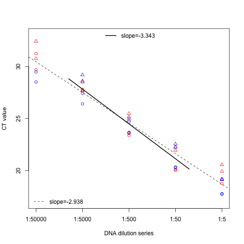

plot of chunk import_data

ps <- subset(df, MM=="SYBR Green")
ps2 <- subset(ps, conc!=2e-01)
mod <- lm(CT ~ log10(conc), data=ps2)
summary(mod)

## 
## Call:
## lm(formula = CT ~ log10(conc), data = ps2)
## 
## Residuals:
##      Min       1Q   Median       3Q      Max 
## -1.40873 -0.88072 -0.02075  0.76958  1.31966 
## 
## Coefficients:
##             Estimate Std. Error t value Pr(>|t|)    
## (Intercept)  15.4057     0.6956   22.15 2.69e-12 ***
## log10(conc)  -3.3394     0.2053  -16.27 1.73e-10 ***
## ---
## Signif. codes:  0 '***' 0.001 '**' 0.01 '*' 0.05 '.' 0.1 ' ' 1
## 
## Residual standard error: 0.9179 on 14 degrees of freedom
## Multiple R-squared:  0.9498,	Adjusted R-squared:  0.9462 
## F-statistic: 264.7 on 1 and 14 DF,  p-value: 1.729e-10

xyplot(CT ~ log10(conc), type=c("r", "p"), data=ps2)

## Error in eval(expr, envir, enclos): could not find function "xyplot"

((10^(-1/coef(mod)[2]))-1)*100

## log10(conc) 
##    99.27435

Based on these results, we can conclude: 1) Pax-C primers amplify target successfully with ~100% efficiency 2) KI Platygyra samples have some PCR inhibitors, but effect disappears after 1:50 dilution 3) There is no advantage of the PowerUp SYBR Mix unless using un-diluted DNA (i.e., at highest level of inhibitors)

Discussion

There is some evidence of minor PCR inhibition, as the Ct values for the highest DNA concentration are slightly higher than expected based on the rest of the dilution series, and the slope of the standard curve including the entire dilution series is -2.938, indicating an amplification efficiency of 118.96% (suggesting inhibition). However, for the middle three levels of the dilution series, the slope is -3.343, indicating an amplification efficiency of 99.13% and no evidence of inhibition. There was no difference in slope between the two MasterMixes used, although at the highest DNA concentration, Ct values were slightly lower for the PowerUp SYBR, indicating it may be slightly more robust to inhibitors at this level. Nevertheless, once samples are diluted tenfold, there is no longer any difference between the two SYBR MasterMixes.

KI samples should be diluted more than 1:5 prior to being assayed with qPCR. Next steps: Test some KI samples that have very low DNA concentrations.